Details:
Published: Feb. 12, 2018
Masking, Visualizing, and Plotting AppEEARS Output GeoTIFF Time Series
This tutorial demonstrates how to use Python to explore time series data in GeoTIFF format generated from the Application for Extracting and Exploring Analysis Ready Samples (AppEEARS) Area Sampler.
AppEEARS allows users to select GeoTIFF as an output file format for Area Requests. This tutorial provides step-by-step instructions for how to filter data in AppEEARS based on specific quality indicators and land cover types, re-create AppEEARS output visualizations and statistics, and generate additional plots to visualize time series data in Python.
Case Study: An Analysis of Field Crop Yield Estimates vs. MODIS Enhanced Vegetation Index (EVI) Data
Reference:
Johnson, D. M. (2016). A comprehensive assessment of the correlations between field crop yields and commonly used MODIS products. International Journal of Applied Earth Observation and Geoinformation, 52, 65-81, https://doi.org/10.1016/j.jag.2016.05.010.
What: The study provides an assessment of correlations between field crop yield estimates and MODIS products.
Why: To explore the range of temperature and vegetation products available at regional-scale (MODIS) to document the relationships between remotely sensed measurements and yield for a variety of crop types.
How: The study analyzed correlation and timing of several MODIS products against field crop yields for ten crops at the county-level.
Where: Conterminous United States, MODIS Tiles: h09-v04,v05,v06; h10-v04,v05,v06; h11-v04,v05
When: April-October 2008-2013
AppEEARS Request Parameters:
- Date (Recurring): April 16 to October 16, 2008-2013
- Data layers:
- Terra MODIS Vegetation Indices
- MOD13Q1.006, 250m, 16 day: '_250m_16_days_EVI'
- Combined MODIS Land Cover Type
- MCD12Q1.051, 500m, Yearly: 'Land_Cover_Type_1'
- Location: Iowa, United States
- Output File Format: GeoTIFF
- Output Projection: Geographic (EPSG: 4326)
Field Crop Yield Estimates Request Parameters: This tutorial uses annual crop yields statistics from the United States Department of Agriculture National Agricultural Statistics Service (USDA NASS). The statistics used include annual surveys of corn and soybean yields by year for the state of Iowa, with yield measured in BU/Acre. The data are available for download through the QuickStats platform.
Topics Covered:
- Getting Started
1a. Setting Up the Working Environment
1b. Opening a GeoTIFF (.tif) File
1c. Reading GeoTIFF Metadata
1d. Applying Scale Factors - Filtering Data
2a. Reading Quality Lookup Tables (LUTs) from CSV Files
2b. Masking by Quality
2c. Masking by Land Cover Type - Visualizations and Statistics
3a. Visualizing GeoTIFF Files
3b. Generating Statistics
3c. Visualizing Statistics - Working with Time Series (Automation)
4a. Batch Processing
4b. Visualizing MODIS Time Series
4c. Generating Statistics
4d. Visualizing Statistics
4e. Exporting Masked GeoTIFF Files
AppEEARS Information:
To access AppEEARS, visit: https://appeears.earthdatacloud.nasa.gov/
For information on how to make an AppEEARS request, visit: https://appeears.earthdatacloud.nasa.gov/help
Statistics:
The statistics covered in this tutorial are the same as the statistics available in AppEEARS. These include box plot statistics, such as the total number of values/pixels (n), the median, and the interquartile range (IQR) of the sample data for values within a feature from a selected date/layer. Also calculated are the Lower 1.5 IQR, which represent the lowest datum still within 1.5 IQR of the lower quartile, and the Upper 1.5 IQR, which represent the highest datum still within 1.5 IQR of the upper quartile. Additional statistics generated for each layer/observation/feature combination include min/max/range, mean, standard deviation, and variance. Frequency distributions also will be calculated for the categorical land cover type 1 layer.
Files Used in this Tutorial:
- JSON file (right-click -> save as -> add extension
.json) - MCD12Q1.051 GeoTIFF Files
- MOD13Q1.006 GeoTIFF Files
- MOD13Q1.006 Quality Lookup Table
- USDA NASS Crop Yields Data
Source Code used to Generate this Tutorial:
**NOTE: Be aware that any reprojection of data from its source projection to a different projection will inherently change the data from its original format. All reprojections use the GDAL gdalwarp function with the PROJ.4 string listed above. For additional information, see the AppEEARS help documentation. **
1. Getting Started
Import the python libraries needed to run this tutorial. If you are missing a package, you will need to download it to execute the notebook.
# Import libraries
import os
import glob
from osgeo import gdal
import numpy as np
import matplotlib.pyplot as plt
import scipy.ndimage
import pandas as pd
import datetime as dt
1a. Setting Up the Working Environment
Next, set your input/working directory, and create an output directory for the results.
# Set input directory, and change working directory
inDir = 'C:/Users/ckrehbiel/Documents/appeears-tutorials/GeoTIFF/'            # IMPORTANT: Update to reflect directory on your OS
os.chdir(inDir)                                                               # Change to working directory
outDir = os.path.normpath(os.path.split(inDir)[0] + os.sep + 'output') + '\\' # Create and set output directory
if not os.path.exists(outDir): os.makedirs(outDir)
1b. Opening a GeoTIFF (.tif) File
You will need to download the MOD13Q1.006 and MCD12Q1.051 zip files and unzip them into the inDir directory to follow along in the tutorial.
Search for the GeoTIFF files in the working directory, create a list of the files, and print the list of MCD12Q1.051 files.
EVIFiles = glob.glob('MOD13Q1.006__250m_16_days_EVI_**.tif') # Search for and create a list of EVI files
LCTFiles =  glob.glob('MCD12Q1.051_Land_Cover_Type**.tif')   # Search for and create a list of LCT files
LCTFiles
['MCD12Q1.051_Land_Cover_Type_1_doy2008001_aid0001.tif',
 'MCD12Q1.051_Land_Cover_Type_1_doy2009001_aid0001.tif',
 'MCD12Q1.051_Land_Cover_Type_1_doy2010001_aid0001.tif',
 'MCD12Q1.051_Land_Cover_Type_1_doy2011001_aid0001.tif',
 'MCD12Q1.051_Land_Cover_Type_1_doy2012001_aid0001.tif',
 'MCD12Q1.051_Land_Cover_Type_1_doy2013001_aid0001.tif']
The products used here include the version 5.1 MODIS Combined Yearly Land Cover Type 1 (MCD12Q1.051) and version 6 MODIS Terra 16-day Vegetation Indices (MOD13Q1.006) products. Start with the first MOD13Q1.006 GeoTIFF file.
Notice below that the list index for EVIFiles is set to 0, indicating that we want the first file in the list. Read the file in by calling the Open() function from the Geospatial Data Abstraction library (GDAL).
EVI = gdal.Open(EVIFiles[0])                    # Read file in, starting with MOD13Q1 version 6
EVIBand = EVI.GetRasterBand(1)                  # Read the band (layer)
EVIData = EVIBand.ReadAsArray().astype('float') # Import band as an array with type float
1c. Reading GeoTIFF Metadata
Below, read the metadata in the GeoTIFF file. Start by using the AppEEARS output filename for some basic metadata.
print(EVIFiles[0])
MOD13Q1.006__250m_16_days_EVI_doy2008113_aid0001.tif
Above is an example of an AppEEARS Output file name. The standard format is as follows:
Product.Version_layer_doyYYYYDDD_aid#####.tif
Below, use the split() function to split the AppEEARS filename string into product.version, layer, area id (aid) and date of the observation, converting from YYYYDDD to MM/DD/YYYY.
# File name metadata:
productId = EVIFiles[0].split('_')[0]                                          # First: product name
layerId = EVIFiles[0].split(productId + '_')[1].split('_doy')[0]               # Second: layer name
yeardoy = EVIFiles[0].split(layerId+'_doy')[1].split('_aid')[0]                # Third: date
aid = EVIFiles[0].split(yeardoy+'_')[1].split('.tif')[0]                       # Fourth: unique ROI identifier (aid)
date = dt.datetime.strptime(yeardoy, '%Y%j').strftime('%m/%d/%Y')              # Convert YYYYDDD to MM/DD/YYYY
print('Product Name: {}\nLayer Name: {}\nDate of Observation: {}'.format(productId, layerId, date))
Product Name: MOD13Q1.006
Layer Name: _250m_16_days_EVI
Date of Observation: 04/22/2008
Below, use the GDAL function GetMetadata() to read the metadata stored within the GeoTIFF file. Store the information as variables to be used at the end of the tutorial for exporting the masked arrays back to GeoTIFF files.
# File Metadata
EVI_meta = EVI.GetMetadata()                   # Store metadata in dictionary
rows, cols = EVI.RasterYSize, EVI.RasterXSize  # Number of rows,columns

# Projection information
geotransform = EVI.GetGeoTransform()
proj= EVI.GetProjection()

# Band metadata
EVIFill = EVIBand.GetNoDataValue()            # Returns fill value
EVIStats = EVIBand.GetStatistics(True, True)  # returns min, max, mean, and standard deviation
EVI = None                                    # Close the GeoTIFF file
print('Min EVI: {}\nMax EVI: {}\nMean EVI: {}\nSD EVI: {}'.format(EVIStats[0],EVIStats[1], EVIStats[2], EVIStats[3]))
Min EVI: -1002.0
Max EVI: 7570.0
Mean EVI: 2097.7074928952597
SD EVI: 960.9360144243974
Notice above that the EVI data are unscaled.
1d. Applying Scale Factors
Next, search for the scale factor in the metadata and apply it to the unscaled array.
scaleFactor = float(EVI_meta['scale_factor'])  # Search the metadata dictionary for the scale factor
units = EVI_meta['units']                      # Search the metadata dictionary for the units
EVIData[EVIData == EVIFill] = np.nan           # Set the fill value equal to NaN for the array
EVIScaled = EVIData * scaleFactor              # Apply the scale factor using simple multiplication

# Generate statistics on the scaled data
EVIStats_sc = [np.nanmin(EVIScaled), np.nanmax(EVIScaled), np.nanmean(EVIScaled), np.nanstd(EVIScaled)] # Create a list of stats
print('Min EVI: {}\nMax EVI: {}\nMean EVI: {}\nSD EVI: {}'.format(EVIStats_sc[0],EVIStats_sc[1], EVIStats_sc[2], EVIStats_sc[3]))
Min EVI: -0.1277
Max EVI: 0.8963000000000001
Mean EVI: 0.21003303941694598
SD EVI: 0.09669416460347872
Above, notice the statistics have changed and appear to fall within a normal distribution (-1 to 1) for EVI values.
2. Filtering Data
2a. Reading Quality Lookup Tables (LUTs) from CSV Files
In this section, take the quality lookup table (LUT) CSV file from an AppEEARS request, read it into Python using the pandas library, and use it to help set the custom quality masking parameters.
The quality LUT for your request (files ending in lookup.csv) can be found under Supporting Files on the Download Area Sample page:
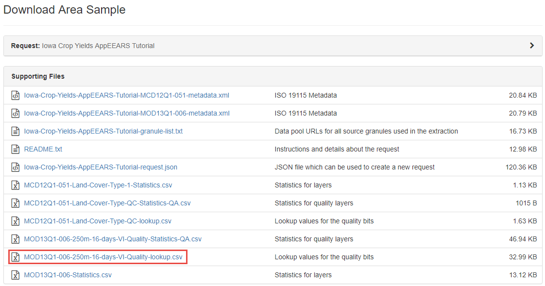
For more information on how to retrieve the quality LUTs from your request, visit the AppEEARS help pages, under Area Samples -> Downloading Your Request.
Once you have saved the MOD13Q1.006 Quality Lookup Table to the inDir directory, search the directory for the LUT and VI Quality GeoTIFFs.
lut = glob.glob('**lookup.csv')                                        # Search for look up table
qualityFiles =glob.glob('MOD13Q1.006__250m_16_days_VI_Quality**.tif')  # Search the directory for the associated quality .tifs
quality = gdal.Open(qualityFiles[0])                                   # Open the first quality file
qualityData = quality.GetRasterBand(1).ReadAsArray()                   # Read in as an array
quality = None                                                         # Close the quality file
Below, use the read_csv function from the pandas library to read the CSV file in as a pandas dataframe.
v6_QA_lut = pd.read_csv(lut[0])     # Read in the lut
v6_QA_lut.head()                    # print the first few rows of the pandas dataframe
| Value | MODLAND | VI Usefulness | Aerosol Quantity | Adjacent cloud detected | Atmosphere BRDF Correction | Mixed Clouds | Land/Water Mask | Possible snow/ice | Possible shadow | |
|---|---|---|---|---|---|---|---|---|---|---|
| 0 | 2057 | VI produced, but check other QA | Decreasing quality | Climatology | No | No | No | Land (Nothing else but land) | No | No |
| 1 | 2058 | Pixel produced, but most probably cloudy | Decreasing quality | Climatology | No | No | No | Land (Nothing else but land) | No | No |
| 2 | 2061 | VI produced, but check other QA | Decreasing quality | Climatology | No | No | No | Land (Nothing else but land) | No | No |
| 3 | 2062 | Pixel produced, but most probably cloudy | Decreasing quality | Climatology | No | No | No | Land (Nothing else but land) | No | No |
| 4 | 2112 | VI produced with good quality | Highest quality | Low | No | No | No | Land (Nothing else but land) | No | No |
Above shows the quality information contained in the LUT. "Value" refers to the pixel value, followed by each specific bit-word beginning with MODLAND. AppEEARS decodes each binary quality bit-field into more meaningful information for the user.
2b. Masking by Quality
This section demonstrates how to take the list of quality values imported above, and mask the quality and EVI arrays to include only pixels where the quality value is in the list of 'good quality' values based on the parameters defined below.
Quality parameters used to define the masking process:
1. MODLAND = 0 or 1
0 = good quality
1 = check other QA
2. VI usefulness <= 11
0000    Highest quality = 0
0001    Lower quality = 1
0010    Decreasing quality = 2
...
1011   Decreasing quality = 11
3. Adjacent cloud detected, Mixed Clouds, and Possible shadow = 0
0 = No
4. Aerosol Quantity = 1 or 2
1 = low aerosol
2 = average aerosol
Below, use the pixel quality flag parameters outlined above to filter the data. Pandas makes this easier by allowing you to search the dataframe by column and value, and only keep the specific values that relate to the parameters desired.
# Include good quality based on MODLAND
v6_QA_lut = v6_QA_lut[v6_QA_lut['MODLAND'].isin(['VI produced with good quality', 'VI produced, but check other QA'])]

# Exclude lower quality VI usefulness
VIU =["Lowest quality","Quality so low that it is not useful","L1B data faulty","Not useful for any other reason/not processed"]
v6_QA_lut = v6_QA_lut[~v6_QA_lut['VI Usefulness'].isin(VIU)]

v6_QA_lut = v6_QA_lut[v6_QA_lut['Aerosol Quantity'].isin(['Low','Average'])]   # Include low or average aerosol
v6_QA_lut = v6_QA_lut[v6_QA_lut['Adjacent cloud detected'] == 'No' ]           # Include where adjacent cloud not detected
v6_QA_lut = v6_QA_lut[v6_QA_lut['Mixed Clouds'] == 'No' ]                      # Include where mixed clouds not detected
v6_QA_lut = v6_QA_lut[v6_QA_lut['Possible shadow'] == 'No' ]                   # Include where possible shadow not detected
v6_QA_lut
| Value | MODLAND | VI Usefulness | Aerosol Quantity | Adjacent cloud detected | Atmosphere BRDF Correction | Mixed Clouds | Land/Water Mask | Possible snow/ice | Possible shadow | |
|---|---|---|---|---|---|---|---|---|---|---|
| 4 | 2112 | VI produced with good quality | Highest quality | Low | No | No | No | Land (Nothing else but land) | No | No |
| 7 | 2116 | VI produced with good quality | Lower quality | Low | No | No | No | Land (Nothing else but land) | No | No |
| 13 | 2181 | VI produced, but check other QA | Lower quality | Average | No | No | No | Land (Nothing else but land) | No | No |
| 16 | 2185 | VI produced, but check other QA | Decreasing quality | Average | No | No | No | Land (Nothing else but land) | No | No |
| 19 | 2189 | VI produced, but check other QA | Decreasing quality | Average | No | No | No | Land (Nothing else but land) | No | No |
| 66 | 4160 | VI produced with good quality | Highest quality | Low | No | No | No | Ocean coastlines and lake shorelines | No | No |
| 69 | 4164 | VI produced with good quality | Lower quality | Low | No | No | No | Ocean coastlines and lake shorelines | No | No |
| 72 | 4168 | VI produced with good quality | Decreasing quality | Low | No | No | No | Ocean coastlines and lake shorelines | No | No |
| 75 | 4229 | VI produced, but check other QA | Lower quality | Average | No | No | No | Ocean coastlines and lake shorelines | No | No |
| 78 | 4233 | VI produced, but check other QA | Decreasing quality | Average | No | No | No | Ocean coastlines and lake shorelines | No | No |
| 119 | 6208 | VI produced with good quality | Highest quality | Low | No | No | No | Shallow inland water | No | No |
| 122 | 6212 | VI produced with good quality | Lower quality | Low | No | No | No | Shallow inland water | No | No |
| 125 | 6216 | VI produced with good quality | Decreasing quality | Low | No | No | No | Shallow inland water | No | No |
| 129 | 6277 | VI produced, but check other QA | Lower quality | Average | No | No | No | Shallow inland water | No | No |
| 131 | 6281 | VI produced, but check other QA | Decreasing quality | Average | No | No | No | Shallow inland water | No | No |
Next, demonstrate how to take the list of possible values (based on table of good quality values above), and mask the quality array. Ultimately, use the masked quality array to mask the EVI array to include only pixels where the quality value is in the list of 'good quality' values.
goodQuality = list(v6_QA_lut['Value']) # Retrieve list of possible QA values from the quality dataframe
print(goodQuality)
[2112, 2116, 2181, 2185, 2189, 4160, 4164, 4168, 4229, 4233, 6208, 6212, 6216, 6277, 6281]
So above, only pixels with those specific _250m_16_days_VI_Quality values will be included after masking.
Below, mask the EVI array using the quality mask. Notice that invert is set to "True" here, meaning that you do not want to exclude the list of values above, but rather exclude all other values.
EVI_masked = np.ma.MaskedArray(EVIScaled, np.in1d(qualityData, goodQuality, invert = True)) # Apply QA mask to the EVI data
2c. Masking by Land Cover Type
Now, take the quality filtered data and apply a mask by land cover type, only keeping those pixels defined as 'croplands' in the MCD12Q1.051 Land Cover Type 1 file. We use Scipy to resample the LCT array (500 m resolution) down to 250 m resolution to match the MOD13Q1.006 EVI array.
LCT = gdal.Open(LCTFiles[0])                              # Open the 2008 land cover type 1 file
LCTData = LCT.GetRasterBand(1).ReadAsArray()              # Read the file as an array
year =LCTFiles[0].split('_doy')[1].split('_aid')[0][0:4]  # Grab the year from the file name
LCT_resampled = scipy.ndimage.zoom(LCTData, 2, order=0)   # Resample by a factor of 2 with nearest neighbor interpolation

# Cropland =12 for Land Cover Type 1 (https://lpdaac.usgs.gov/dataset_discovery/modis/modis_products_table/mcd12q1)
cropland = 12

# Resampling leads to 1 extra row and column, so delete first row and last column to align arrays
LCT_resampled = np.delete(LCT_resampled, 0, 0)
LCT_resampled = np.delete(LCT_resampled, 3121, 1)
EVI_crops = np.ma.MaskedArray(EVI_masked, np.in1d(LCT_resampled, cropland, invert = True)) # Mask array, only include Croplands
LCT = None                                                                                 # Close the file
3. Visualization and Statistics
# Set matplotlib plots inline
%matplotlib inline
3a. Visualizing GeoTIFF Files
In this section, begin by highlighting the functionality of the matplotlib plotting package. First, make a basic plot of the EVI data. Next, add some additional parameters to the plot. Finally, export the completed plot to an image file.
plt.imshow(EVIScaled); # Visualize a basic plot of the scaled EVI data
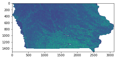
Above, adding ; to the end of the call suppresses the text output from appearing in the notebook. The output is a basic matplotlib plot of the scaled EVI array showing the state of Iowa, United States.
Next, add some additional parameters to the visualization.
plt.figure(figsize = (10,7.5))    # Set the figure size (x,y)
plt.axis('off')                   # Remove the axes' values

# Plot the array, using a colormap and setting a custom linear stretch based on the min/max EVI values
plt.imshow(EVIScaled, vmin = np.nanmin(EVIScaled), vmax = np.nanmax(EVIScaled), cmap = 'YlGn');
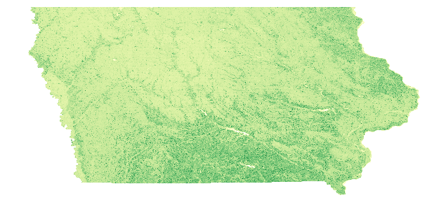
Above, notice a better visual representation of the data. However, it still is missing important items, such as a title and a colormap legend.
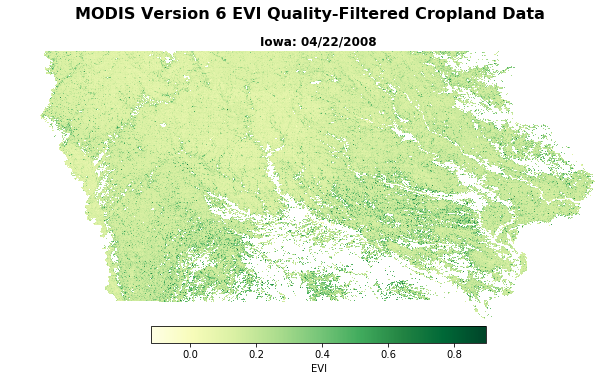
Plot the quality-filtered, land cover-masked EVI array, add a title/subtitle and colormap legend, and export to a .png file in the output directory.
fig = plt.figure(figsize=(10,6.5))                                                                 # Set the figure size
plt.axis('off')                                                                                    # Remove the axes' values
fig.suptitle('MODIS Version 6 EVI Quality-Filtered Cropland Data', fontsize=16, fontweight='bold') # Make a figure title
ax = fig.add_subplot(111)                                                                          # Make a subplot
fig.subplots_adjust(top=3.8)                                                                       # Adjust spacing
ax.set_title('Iowa: {}'.format(date), fontsize=12, fontweight='bold')                              # Add figure subtitle
ax1 = plt.gca()                                                                                    # Get current axes

# Plot the masked data, using a colormap and setting a custom linear stretch based on the min/max EVI values
im = ax1.imshow(EVI_crops, vmin=EVI_crops.min(), vmax=EVI_crops.max(), cmap='YlGn');

# Add a colormap legend
plt.colorbar(im, orientation='horizontal', fraction=0.047, pad=0.004, label='EVI', shrink=0.6).outline.set_visible(True)

# Set up file name and export to png file
fig.savefig('{}{}.png'.format(outDir, (EVIFiles[0].split('.tif'))[0]), bbox_inches='tight')
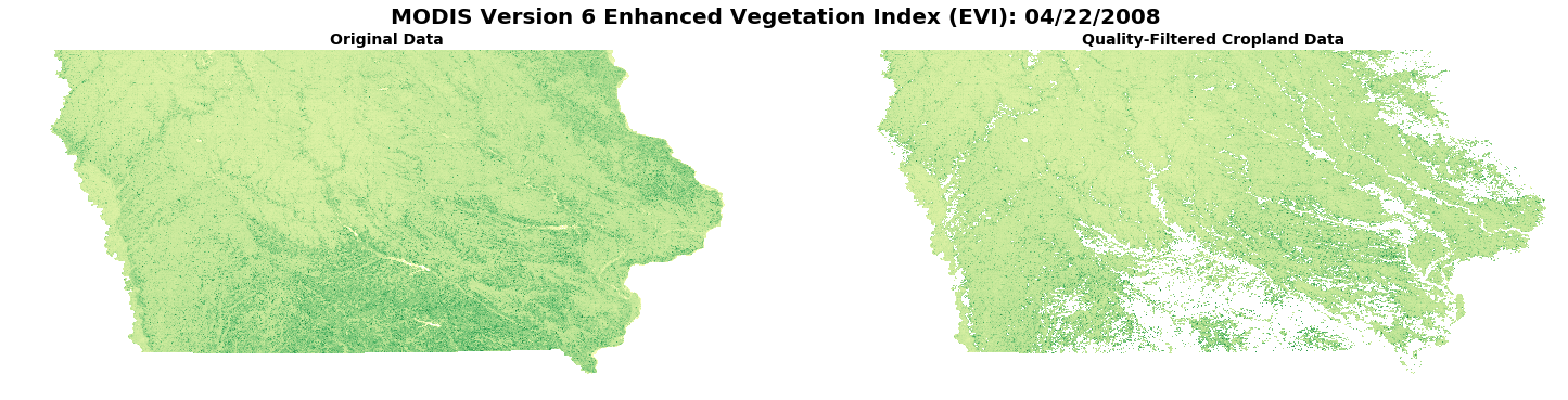
Next, set multiple plots to compare original versus quality-masked croplands-only data.
figure, axes = plt.subplots(nrows=1, ncols=2, figsize=(25, 5.5), sharey=True, sharex=True) # Set subplots with 1 row & 2 columns
axes[0].axis('off'), axes[1].axis('off')                                                   # Turn off axes' values

# Add a title for the plots
figure.suptitle('MODIS Version 6 Enhanced Vegetation Index (EVI): {}'.format(date), fontsize=20, fontweight='bold')

axes[0].set_title('Original Data', fontsize=14, fontweight='bold')                  # Set the first subplot title
axes[1].set_title('Quality-Filtered Cropland Data', fontsize=14, fontweight='bold') # Set the second subplot title
axes[0].imshow(EVIScaled, vmin=-0.2, vmax=1.0, cmap='YlGn');                        # Plot original data
axes[1].imshow(EVI_crops, vmin=-0.2, vmax=1.0, cmap='YlGn');                        # Plot Quality-filtered data
3b. Generating Statistics
Below, calculate a variety of statistics available in AppEEARS. Begin by making an array that only includes quality-filtered, cropland pixels.
EVI_crops2 = EVI_crops.data[~EVI_crops.mask]    # Exclude non-cropland pixel values
EVI_crops2 = EVI_crops2[~np.isnan(EVI_crops2)]  # Exclude poor quality pixel values
Below, use Numpy functions to calculate statistics on the quality-masked, croplands-only data. The format( , '4f') command will ensure that the statistics are rounded to four decimal places (same number as AppEEARS output statistics).
n = len(EVI_crops2)                                                        # Count of array
min_val = float(format((np.min(EVI_crops2)), '.4f'))                       # Minimum value in array
max_val = float(format((np.max(EVI_crops2)), '.4f'))                       # Maximum value in array
range_val = (min_val, max_val)                                             # Range of values in array
mean = float(format((np.mean(EVI_crops2)), '.4f'))                         # Mean of values in array
std = float(format((np.std(EVI_crops2)), '.4f'))                           # Standard deviation of values in array
var = float(format((np.var(EVI_crops2)), '.4f'))                           # Variance of values in array
median = float(format((np.median(EVI_crops2)), '.4f'))                     # Median of values in array
quartiles = np.percentile(EVI_crops2, [25, 75])                            # 1st (25) and 3rd (75) quartiles of values in array
upper_quartile = float(format((quartiles[1]), '.4f'))
lower_quartile = float(format((quartiles[0]), '.4f'))
iqr = quartiles[1] - quartiles[0]                                          # Interquartile range
iqr_upper = upper_quartile + 1.5 * iqr                                     # 1.5 IQR of the upper quartile
iqr_lower = lower_quartile - 1.5 * iqr                                     # 1.5 IQR of the lower quartile
top = float(format(np.max(EVI_crops2[EVI_crops2 <= iqr_upper]), '.4f'))    # Highest datum still within 1.5 IQR of upper quartile
bottom = float(format(np.min(EVI_crops2[EVI_crops2 >= iqr_lower]), '.4f')) # Lowest datum still within 1.5 IQR of lower quartile
Next, set up a dictionary with names (keys) for each statistic calculated above, and assign each statistic to the correct name (key).
d = {'File Name':(EVIFiles[0]), 'Dataset': layerId, 'aid': aid, 'Date': date, 'Count':n, 'Minimum':min_val, 'Maximum':max_val,
     'Range':range_val, 'Mean':mean, 'Median':median, 'Upper Quartile':upper_quartile, 'Lower Quartile':lower_quartile,
     'Upper 1.5 IQR':top, 'Lower 1.5 IQR':bottom, 'Standard Deviation':std, 'Variance':var}
for dd in d: print(dd + ' = ' + str(d[dd]))  # Print the results from calculating statistics
File Name = MOD13Q1.006__250m_16_days_EVI_doy2008113_aid0001.tif
Dataset = _250m_16_days_EVI
aid = aid0001
Date = 04/22/2008
Count = 2921041
Minimum = -0.1168
Maximum = 0.8963
Range = (-0.1168, 0.8963)
Mean = 0.1871
Median = 0.1649
Upper Quartile = 0.2115
Lower Quartile = 0.1358
Upper 1.5 IQR = 0.325
Lower 1.5 IQR = 0.0224
Standard Deviation = 0.0807
Variance = 0.0065
Now set up a pandas dataframe to store the statistics and import the statistics from the dictionary created above.
# Create dataframe
stats_df = pd.DataFrame(columns=['File Name', 'Dataset', 'aid', 'Date', 'Count', 'Minimum', 'Maximum', 'Range', 'Mean','Median',
                        'Upper Quartile', 'Lower Quartile', 'Upper 1.5 IQR', 'Lower 1.5 IQR', 'Standard Deviation', 'Variance'])
stats_df = stats_df.append(d, ignore_index=True) # Append the dictionary to the dataframe
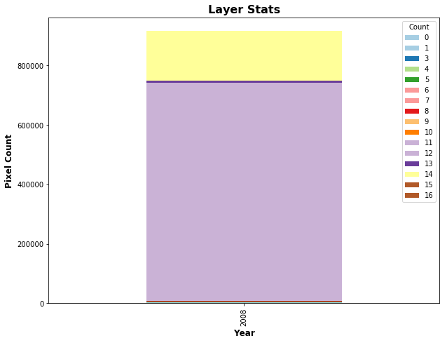
Below, calculate and print the frequency distribution of land cover type 1 values from 2008 in Iowa.
LCTData = LCTData[LCTData!=255]                    # Exclude fill value
freq_dist = np.unique(LCTData, return_counts=True) # find the unique values in the LCT array and return counts

for i in range(len(freq_dist[0])):print('Value: {}, Count: {}'.format(freq_dist[0][i], freq_dist[1][i]))  # Print values/counts
Value: 0, Count: 1547
Value: 1, Count: 1017
Value: 3, Count: 191
Value: 4, Count: 1456
Value: 5, Count: 2231
Value: 6, Count: 117
Value: 7, Count: 3
Value: 8, Count: 668
Value: 9, Count: 24
Value: 10, Count: 880
Value: 11, Count: 1038
Value: 12, Count: 733121
Value: 13, Count: 5660
Value: 14, Count: 168219
Value: 15, Count: 1
Value: 16, Count: 125
3c. Visualizing Statistics
Below, recreate similar boxplots and bar charts to those available in the AppEEARS UI using the Matplotlib package.
plt.boxplot(EVI_crops2); # Basic boxplot
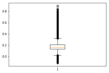
Above is a very basic matplotlib boxplot.
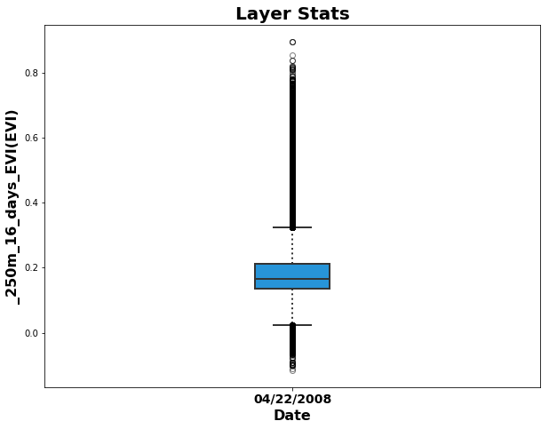
Below, add important items such as a title, different colors, and labels.
fig = plt.figure(1, figsize=(10, 7.5))            # Set the figure size
ax = fig.add_subplot(111)                         # Create a subplot
box = ax.boxplot(EVI_crops2, patch_artist=True);  # Add the boxplot of quality-filtered, croplands-only data

# Set boxplot attributes similar to the AppEEARS UI.
for b in box['boxes']: b.set( color='#333333', linewidth=2), b.set(facecolor='#2794D8')  # Set box outline and fill color
for m in box['medians']: m.set(color='#333333', linewidth=2)                             # Set color/linewidth of medians
for w in box['whiskers']: w.set(color='#333333', linewidth=2), w.set_linestyle(':')      # Set color/linewidth of whiskers
for c in box['caps']: c.set(color='#333333', linewidth=2)                                # Set color/linewidth of caps
for f in box['fliers']: f.set(marker='o', color='#cccccc', alpha=0.5)                    # Set the style of fliers
ax.set_xticklabels([date],fontsize=14, fontweight='bold')                                # Add date to x-axis
ax.set_xlabel('Date', fontsize=16, fontweight='bold')                                    # Add label to x-axis
ax.set_ylabel("{}({})".format(layerId, units), fontsize=16, fontweight='bold')           # Add label/units to y-axis
ax.set_title('Layer Stats', fontsize=20, fontweight='bold');                             # Add title
For additional information on how to create boxplots with matplotlib, see: http://blog.bharatbhole.com/creating-boxplots-with-matplotlib/.
For categorical layers, such as land cover type 1, AppEEARS creates stacked bar charts, shown below.
# Add stacked bar chart
n = len(np.unique(LCTData))                             # Get the number of unique values in the LCT array
LCTchart = [[year]*n, freq_dist[0], freq_dist[1]]       # Create an array with year, values, and counts
row = list(zip(LCTchart[0], LCTchart[1], LCTchart[2]))  # Zip the data together
headers = ['Year', 'Count', 'Value']                    # Set the headers

# Use the pivot function to reconfigure data for plotting
lct_df = pd.DataFrame(row, columns=headers).pivot(index='Year', columns='Count', values='Value')
ax = lct_df.loc[:,freq_dist[0]].plot.bar(stacked=True,colormap='Paired',figsize=(10,7.5),title='Layer Stats'); # Reorder layers


# Add a title and x/y labels
ax.set_ylabel("Pixel Count", fontsize=12, fontweight='bold');  # Add y-axis label
ax.set_xlabel('Year', fontsize=12, fontweight='bold');         # Add x-axis label
ax.set_title('Layer Stats', fontsize=16, fontweight='bold');   # Add title
For more information on how to configure stacked bar charts with matplotlib and pandas, see: https://pstblog.com/2016/10/04/stacked-charts.
# Delete variables that will not be needed in the next section
del LCTData, freq_dist, EVI_crops2, LCTchart, axes, dd, headers, i, n, lct_df, row, stats_df, min_val, max_val
del range_val, mean, std, var, median, quartiles, upper_quartile, lower_quartile, iqr, iqr_upper, iqr_lower, top, bottom
del EVI_crops,  EVIScaled, EVI_masked, v6_QA_lut, VIU, lut, EVIStats_sc, EVI_meta, EVIStats, d, box
4. Working with Time Series (Automation)
Here, automate some of the steps above to get multiple growing seasons worth of data for visualization and statistical analysis.
print('Loop through and process {} files in the time series.'.format(len(EVIFiles)))
Loop through and process 72 files in the time series.
4a. Batch Processing
Begin by reconfiguring the original EVI and quality arrays to include a third dimension, which we will ultimately use to stack multiple observations into a three-dimensional array.
date = list([date])                       # Convert from string to a list
EVIData = EVIData[np.newaxis,:,:]         # Add a third axis for stacking rasters
qData = qualityData[np.newaxis,:,:]       # Add a third axis for stacking rasters
del qualityData
Use a for loop to iterate through the remaining 71 EVI files. First, open the next EVI file and corresponding quality layer in chronological order, read in as an array, add the third axis, and use the Numpy library function np.append to combine each file into a multi-dimensional array.
# Loop through and perform processing steps for all 72 EVI and corresponding quality layers
for i in range(1, len(EVIFiles)):
    EVI, q = gdal.Open(EVIFiles[i]), gdal.Open(qualityFiles[i])                                   # Read files in
    EVIb,qb = EVI.GetRasterBand(1).ReadAsArray().astype('float'),q.GetRasterBand(1).ReadAsArray() # Read layers, import as array
    EVIb, qb = EVIb[np.newaxis,:,:], qb[np.newaxis,:,:]                                           # Add a third axis
    EVIData, qData = np.append(EVIData, EVIb, axis=0), np.append(qData,qb, axis=0)                # Append to 'master' 3d array
    del EVIb, qb                                                                                  # Delete intermediate arrays
    EVI, q = None, None                                                                           # Close files
    yeardoy = EVIFiles[i].split(layerId + '_doy')[1].split('_aid')[0]                             # parse filename for date
    date.append(dt.datetime.strptime(yeardoy,'%Y%j').strftime('%m/%d/%Y'))                        # Add to list of dates
EVIData[EVIData == EVIFill] = np.nan                                                              # If EVI = fill, set to nan
EVIScaled = EVIData * scaleFactor                                                                 # Apply scale factor
del EVIData, yeardoy
To automate land cover masking, first bring in each of the annual Land Cover Type 1 layers and stack into three-dimensional array by year.
LCT_resampled = LCT_resampled[np.newaxis,:,:]  # Add a third axis for first year LCT array from above
year = [year]                                  # Convert string to list to store each year
LCTFiles
['MCD12Q1.051_Land_Cover_Type_1_doy2008001_aid0001.tif',
 'MCD12Q1.051_Land_Cover_Type_1_doy2009001_aid0001.tif',
 'MCD12Q1.051_Land_Cover_Type_1_doy2010001_aid0001.tif',
 'MCD12Q1.051_Land_Cover_Type_1_doy2011001_aid0001.tif',
 'MCD12Q1.051_Land_Cover_Type_1_doy2012001_aid0001.tif',
 'MCD12Q1.051_Land_Cover_Type_1_doy2013001_aid0001.tif']
Loop through and open each of the remaining five (annual) files above and stack into a three-dimensional array.
for i in range(1, len(LCTFiles)):
    LCT = gdal.Open(LCTFiles[i])                                 # Read file in
    LCTb = LCT.GetRasterBand(1).ReadAsArray()                    # Import LCT layer as array
    LCTb = scipy.ndimage.zoom(LCTb, 2, order=0)                  # Resample by a factor of 2 with nearest neighbor interpolation
    LCTb = np.delete(LCTb, 0, 0)                                 # Resampling leads to 1 extra row and column,
    LCTb = np.delete(LCTb, 3121, 1)                              # So delete first row and last column to align arrays
    LCTb = LCTb[np.newaxis,:,:]                                  # Add a third axis
    LCT_resampled = np.append(LCT_resampled,LCTb, axis = 0)      # Append to 'master' 3d array
    del LCTb                                                     # Delete intermediate array
    LCT = None                                                   # Close file
    yeardoy =LCTFiles[i].split('_doy')[1].split('_aid')[0][0:4]  # Parse filename for year
    year.append(yeardoy)                                         # Append to list of years
del LCTFiles, qualityFiles
Next, loop through and use a nested for loop to filter the EVI files by quality and land cover type. The nested for loop is used to loop through each year to mask the EVI data using the corresponding Land Cover Type 1 file by year.
i = 0 # Set up our iterator

# Apply QA mask to the EVI data
for x in range(LCT_resampled.shape[0]):
    for i in range(i,i+12):  # 12 observations per year, so every 12th observation use the next year for LCT masking
        if i == 0:
            EVI_masked = np.ma.MaskedArray(EVIScaled[i],np.in1d(qData[i],goodQuality,invert=True))       # Quality mask
            EVI_crops = np.ma.MaskedArray(EVI_masked,np.in1d(LCT_resampled[x], cropland, invert = True)) # Crop mask
            EVI_crops = EVI_crops[np.newaxis,:,:]                                                        # Add third axis
        else:
            EVI_m = np.ma.MaskedArray(EVIScaled[i], np.in1d(qData[i], goodQuality, invert = True))       # Quality mask
            EVI_c = np.ma.MaskedArray(EVI_m, np.in1d(LCT_resampled[x], cropland, invert = True))         # Crop mask
            EVI_c = EVI_c[np.newaxis,:,:]                                                                # Add third axis
            EVI_crops = np.ma.concatenate((EVI_crops,EVI_c))                                             # Add to master array
            del EVI_m, EVI_c
        i = i + 1
del LCT_resampled, EVIScaled, cropland, goodQuality, qData
4b. Visualizing MODIS Time Series
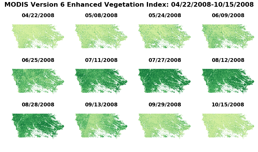
Now, take an entire growing season of quality-filtered croplands-only arrays, and plot together.
figure, axes = plt.subplots(nrows=3, ncols=4, figsize=(15, 8), sharey=True, sharex=True) # Set up subplots w/ 3 rows x 4 columns

# Add a title for the series of plots
figure.suptitle('MODIS Version 6 Enhanced Vegetation Index: {}-{}'.format(date[0],date[11]), fontsize=22, fontweight='bold')

# Set the subplot titles
axes[0][0].set_title(date[0],fontsize=18,fontweight='bold'),axes[0][1].set_title(date[1],fontsize=18,fontweight='bold')
axes[0][2].set_title(date[2],fontsize=18,fontweight='bold'),axes[0][3].set_title(date[3],fontsize=18,fontweight='bold')
axes[1][0].set_title(date[4],fontsize=18,fontweight='bold'),axes[1][1].set_title(date[5],fontsize=18,fontweight='bold')
axes[1][2].set_title(date[6],fontsize=18,fontweight='bold'),axes[1][3].set_title(date[7],fontsize=18,fontweight='bold')
axes[2][0].set_title(date[8],fontsize=18,fontweight='bold'),axes[2][1].set_title(date[9],fontsize=18,fontweight='bold')
axes[2][2].set_title(date[10],fontsize=18,fontweight='bold'),axes[2][3].set_title(date[11],fontsize=18,fontweight='bold')

# Plot each observation
axes[0][0].imshow(EVI_crops[0],vmin=-0.2,vmax=1.0,cmap='YlGn'),axes[0][1].imshow(EVI_crops[1],vmin=-0.2,vmax=1.0,cmap='YlGn')
axes[0][2].imshow(EVI_crops[2],vmin=-0.2,vmax=1.0,cmap='YlGn'),axes[0][3].imshow(EVI_crops[3],vmin=-0.2,vmax=1.0,cmap='YlGn')
axes[1][0].imshow(EVI_crops[4],vmin=-0.2,vmax=1.0,cmap='YlGn'),axes[1][1].imshow(EVI_crops[5],vmin=-0.2,vmax=1.0,cmap='YlGn')
axes[1][2].imshow(EVI_crops[6],vmin=-0.2,vmax=1.0,cmap='YlGn'),axes[1][3].imshow(EVI_crops[7],vmin=-0.2,vmax=1.0,cmap='YlGn')
axes[2][0].imshow(EVI_crops[8],vmin=-0.2,vmax=1.0,cmap='YlGn'),axes[2][1].imshow(EVI_crops[9],vmin=-0.2,vmax=1.0,cmap='YlGn')
axes[2][2].imshow(EVI_crops[10],vmin=-0.2,vmax=1.0,cmap='YlGn'),axes[2][3].imshow(EVI_crops[11],vmin=-0.2,vmax=1.0,cmap='YlGn')

for x in axes.ravel(): x.axis("off") # Remove the axes' values
4c. Generating Statistics
Below, calculate a range of statistics that are available in AppEEARS. First set a pandas dataframe to store the statistics.
# Create dataframe with column names
stats_df = pd.DataFrame(columns=['File Name', 'Dataset', 'aid', 'Date', 'Count', 'Minimum', 'Maximum', 'Range','Mean','Median',
                        'Upper Quartile', 'Lower Quartile', 'Upper 1.5 IQR', 'Lower 1.5 IQR', 'Standard Deviation', 'Variance'])
EVI_all = [] # Create empty list
i = 0        # Set up iterator
Below, use Numpy functions to calculate statistics on the quality-masked, croplands-only data. The format( , '4f') command will ensure that the statistics are rounded to four decimal places (same number as AppEEARS output statistics).
for e in EVI_crops:
    EVI_crops2 = e.data[~e.mask]                                            # Exclude non-cropland pixel values
    EVI_crops2 = EVI_crops2[~np.isnan(EVI_crops2)]                          # Exclude poor quality pixel values
    n = len(EVI_crops2)                                                     # Count of array
    min_val = float(format((np.min(EVI_crops2)), '.4f'))                    # Minimum value in array
    max_val = float(format((np.max(EVI_crops2)), '.4f'))                    # Maximum value in array
    range_val = (min_val, max_val)                                          # Range of values in array
    mean = float(format((np.mean(EVI_crops2)), '.4f'))                      # Mean of values in array
    std = float(format((np.std(EVI_crops2)), '.4f'))                        # Standard deviation of values in array
    var = float(format((np.var(EVI_crops2)), '.4f'))                        # Variance of values in array
    median = float(format((np.median(EVI_crops2)), '.4f'))                  # Median of values in array
    quartiles = np.percentile(EVI_crops2, [25, 75])                         # 1st (25) & 3rd (75) quartiles of values in array
    upper_quartile = float(format((quartiles[1]), '.4f'))
    lower_quartile = float(format((quartiles[0]), '.4f'))
    iqr = quartiles[1] - quartiles[0]                                       # Interquartile range
    iqr_upper = upper_quartile + 1.5 * iqr                                  # 1.5 IQR of the upper quartile
    iqr_lower = lower_quartile - 1.5 * iqr                                  # 1.5 IQR of the lower quartile
    top = float(format(np.max(EVI_crops2[EVI_crops2 <= iqr_upper]), '.4f')) # Highest datum within 1.5 IQR of upper quartile
    bottom = float(format(np.min(EVI_crops2[EVI_crops2>=iqr_lower]),'.4f')) # Lowest datum within 1.5 IQR of lower quartile

    d = {'File Name':(EVIFiles[i]),'Dataset': layerId,'aid': aid,'Date': date[i],'Count':n,'Minimum':min_val,'Maximum':max_val,
         'Range':range_val, 'Mean':mean,'Median':median,'Upper Quartile':upper_quartile,'Lower Quartile':lower_quartile,
         'Upper 1.5 IQR':top, 'Lower 1.5 IQR':bottom,'Standard Deviation':std, 'Variance':var}
    stats_df = stats_df.append(d, ignore_index=True)                        # Append the dictionary to the dataframe
    EVI_all.append([EVI_crops2])                                            # Append to quality-filtered croplands-only array
    i = i + 1
del d, n, min_val, max_val, range_val, mean, std, var, median, quartiles, upper_quartile,
del bottom, EVI_crops2, axes, e, yeardoy, lower_quartile, iqr, iqr_upper, iqr_lower, top
Now, export the results to a csv file in the same style as AppEEARS output statistics CSV files.
stats_df.to_csv('{0}{1}-Statistics.csv'.format(outDir, productId), index = False) # Export statistics to CSV
4d. Visualizing Statistics
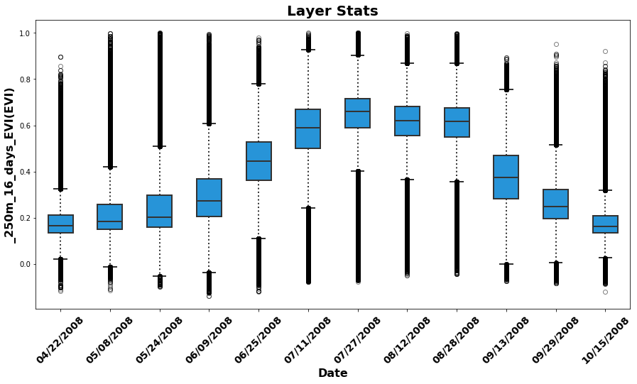
Below, recreate boxplot time series similar to those available in the AppEEARS UI. Later, demonstrate additional plots that can be generated.
Start by plotting a boxplot time series for all observations from 2008.
fig = plt.figure(1, figsize=(15, 7.5))               # Set the figure size
ax = fig.add_subplot(111)                            # Create a subplot
box = ax.boxplot(EVI_all[0:12], patch_artist=True);  # Boxplot of quality-filtered croplands-only data for 1st 12 layers (2008)

# Set boxplot attributes similar the AppEEARS UI
for b in box['boxes']: b.set( color='#333333', linewidth=2), b.set(facecolor='#2794D8')  # Set box outline and fill color
for m in box['medians']: m.set(color='#333333', linewidth=2)                             # Set color/linewidth of medians
for w in box['whiskers']: w.set(color='#333333', linewidth=2), w.set_linestyle(':')      # Set color/linewidth of whiskers
for c in box['caps']: c.set(color='#333333', linewidth=2)                                # Set color/linewidth of caps
for f in box['fliers']: f.set(marker='o', color='#cccccc', alpha=0.5)                    # Set the style of fliers

ax.set_xticklabels(date,fontsize=14, fontweight='bold', rotation=45)                     # Add date to x-axis
ax.set_xlabel('Date', fontsize=16, fontweight='bold')                                    # Add label to x-axis
ax.set_ylabel("{}({})".format(layerId, units), fontsize=16, fontweight='bold')           # Add label/units to y-axis
ax.set_title('Layer Stats', fontsize=20, fontweight='bold');                             # Add title

# Set up file name and export to png file
fig.savefig('{}{}_{}_Boxplot_TimeSeries.png'.format(outDir, productId, layerId), bbox_inches='tight')
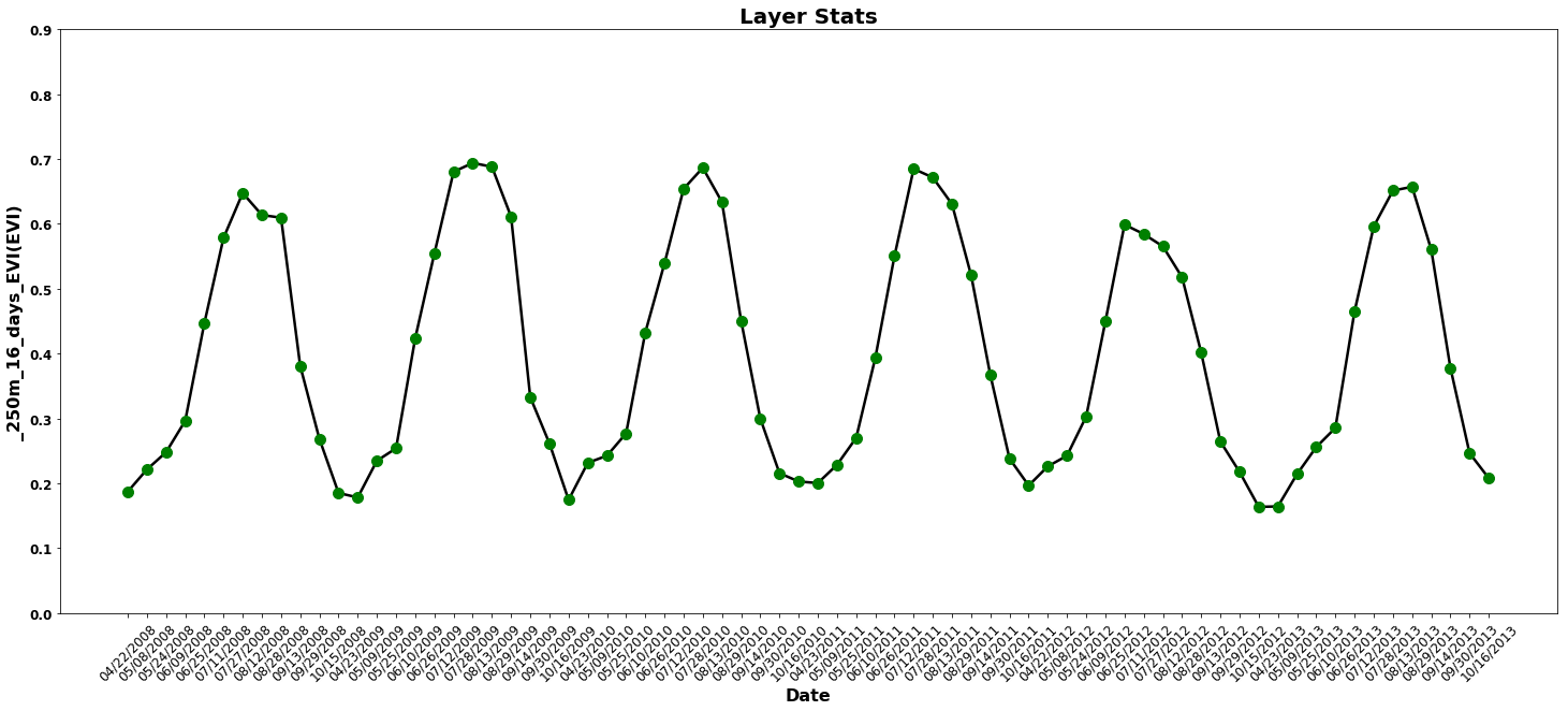
Next, use the previously calculated statistics to plot a time series of Mean EVI for the six year time period.
fig = plt.figure(1, figsize=(25, 10))                                                      # Set the figure size
ax = fig.add_subplot(111)                                                                  # Create a subplot
ax.plot(stats_df['Mean'], 'k', lw=2.5, color='black')                                      # Plot as a black line
ax.plot(stats_df['Mean'], 'bo', ms=10, color='green')                                      # Plot as a green circle
ax.set_xticks((np.arange(0,len(EVIFiles))))                                                # Set the x ticks
ax.set_xticklabels(date, rotation=45,fontsize=12)                                          # Set the x tick labels
ax.set_yticks((np.arange(0,1, 0.1)))                                                       # Arrange the y ticks
ax.set_yticklabels(np.arange(0,1, 0.1),fontsize=12,fontweight='bold')                      # Set the Y tick labels
ax.set_xlabel('Date',fontsize=16,fontweight='bold')                                        # Set x-axis label
ax.set_ylabel("{}({})".format(layerId, units),fontsize=16,fontweight='bold')               # Set y-axis label
ax.set_title('Layer Stats',fontsize=20,fontweight='bold')                                  # Set title
fig.savefig('{}{}_{}_Mean_TS.png'.format(outDir, productId, layerId), bbox_inches='tight') # Set up filename and export
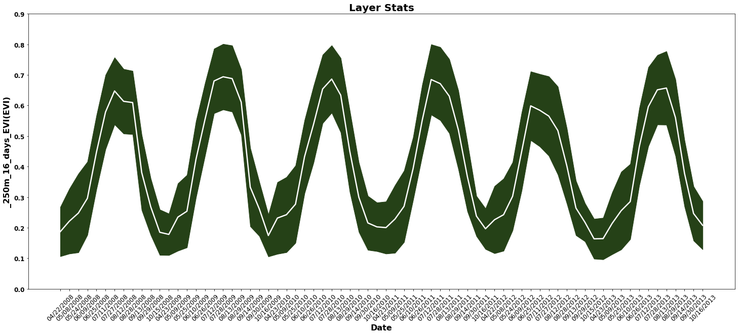
Take the figure one step further, and plot the standard deviation as a confidence interval around the mean EVI as a time series.
fig = plt.figure(1, figsize=(25, 10))  # Set the figure size
dates = np.arange(0,len(EVIFiles),1)   # Arrange all dates
ax = fig.add_subplot(111)              # Add subplot

# Add and subtract the standard deviation from the mean to form the upper and lower intervals for the plot
ax.fill_between(dates,stats_df.Mean-stats_df['Standard Deviation'],stats_df.Mean+stats_df['Standard Deviation'],color='#254117')

ax.plot(stats_df['Mean'], color="white", lw=2.5)                                             # Plot the mean EVI as a white line
ax.set_xticks((np.arange(0,len(EVIFiles))))                                                  # Arrange x ticks
ax.set_xticklabels(date, rotation=45,fontsize=12)                                            # Set x tick labels
ax.set_yticks((np.arange(0,1, 0.1)))                                                         # Arrange y ticks
ax.set_yticklabels(np.arange(0,1, 0.1),fontsize=12,fontweight='bold')                        # Set y-tick labels
ax.set_xlabel('Date',fontsize=16,fontweight='bold')                                          # Set x-axis label
ax.set_ylabel("{}({})".format(layerId, units),fontsize=16,fontweight='bold')                 # Set y-axis label
ax.set_title('Layer Stats',fontsize=20,fontweight='bold')                                    # Add title
fig.savefig('{}{}_{}_MeanStd_TS.png'.format(outDir, productId, layerId),bbox_inches='tight') # Set up filename & export
Below, import annual crop yields statistics from the United States Department of Agriculture National Agricultural Statistics Service (USDA NASS). The statistics used here include annual surveys of corn and soybean yields by year for the state of Iowa, with yield measured in BU/Acre. The data are available for download here through the QuickStats platform.
# Scatterplots: Corn and Soybean yields vs. mean NDVI by year
stats_df['Date2'] = pd.to_datetime(stats_df.Date)                                # Create new df column, convert to datetime
summerstats = stats_df[stats_df.Date2.dt.month !=4]                              # Exclude April obs from mean calculation
summerstats = summerstats[summerstats.Date2.dt.month !=10]                       # Exclude October obs from mean calculation
annualEVI = summerstats.groupby([summerstats.Date2.dt.year])['Mean'].agg('mean') # Calculate 'mean of mean EVI' for May-Sep/year

# Open the crop yields csv file downloaded from the link above
USDA_yields = glob.glob('F750A15B-E3A8-35B9-B688-67FFFBFB1FBF.csv') # will need to change to the specific name of your download
yields = pd.read_csv(USDA_yields[0])                                # Read in the csv file
yields = yields.sort_values(by=['Year'])                            # Sort by year
cornyields = list(yields.Value[yields.Commodity=='CORN'])           # Set corn yields to a variable
soyyields = list(yields.Value[yields.Commodity=='SOYBEANS'])        # Set soybean yields to a variable
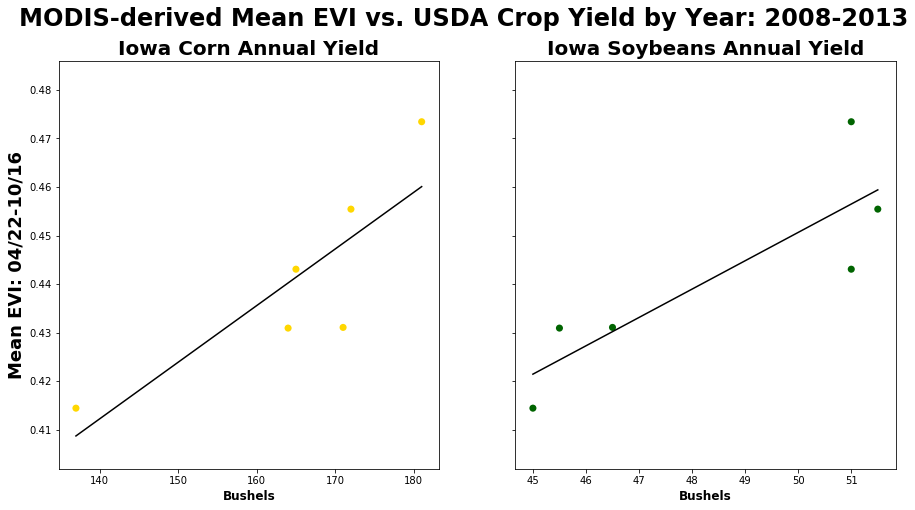
Finally, set up a scatter plot and plot corn/soy yields vs. mean of mean EVI (May-Sept) by year for the state of Iowa.
# Set the figure size -- sharing the y-axis but not the x-axis
figure, axes = plt.subplots(nrows=1, ncols=2, figsize=(15, 7.5), sharey=True, sharex=False)

# Add an overall title for the plots
figure.suptitle('MODIS-derived Mean EVI vs. USDA Crop Yield by Year: 2008-{}'.format(year[-1]),fontsize=24,fontweight='bold')

axes[0].set_title('Iowa Corn Annual Yield',fontsize=20,fontweight='bold')      # Set the title for the first plot
axes[1].set_title('Iowa Soybeans Annual Yield',fontsize=20,fontweight='bold')  # Set the title for the second plot

# Set y and x axes labels
axes[0].set_ylabel('Mean EVI: {}-{}'.format(date[0][0:5],date[len(date)-1][0:5]),fontsize=18,fontweight='bold')
axes[0].set_xlabel('Bushels',fontsize=12,fontweight='bold'), axes[1].set_xlabel('Bushels',fontsize=12,fontweight='bold')

axes[0].scatter(cornyields,annualEVI , alpha=1, c='gold', edgecolors='none', s=50, label="Corn");         # Plot values for corn
axes[1].scatter(soyyields,annualEVI , alpha=1, c='darkgreen', edgecolors='none', s=50, label="Soybeans"); # Plot values for soy

# Plot the linear regression line for corn and soybeans
axes[0].plot(np.unique(cornyields),np.poly1d(np.polyfit(cornyields,annualEVI,1))(np.unique(cornyields)),c='black');
axes[1].plot(np.unique(soyyields), np.poly1d(np.polyfit(soyyields, annualEVI, 1))(np.unique(soyyields)), c ='black');
4e. Exporting Masked GeoTIFFs
Finally, after demonstrating how to filter data, calculate statistics, and create additional visuals, export the masked GeoTIFFs using a for loop.
o = 0 # Set up iterator
for tif in EVI_crops:                                                               # Loop through each array, export to GeoTIFF
    tif.unshare_mask()                                                              # Split mask from data
    tif[tif.mask == True] = EVIFill                                                 # Set masked values equal to fill value
    out_filename ='{}{}_Croplands.tif'.format(outDir,EVIFiles[o].split('.tif')[0])  # Generate output filename
    driver = gdal.GetDriverByName('GTiff')                                          # Select GDAL GeoTIFF driver
    outfile = driver.Create(out_filename, cols, rows, 1, gdal.GDT_Float32)          # Specify the parameters of the GeoTIFF
    outfile.SetGeoTransform(geotransform)                                           # Set Geotransform
    band = outfile.GetRasterBand(1)                                                 # Get band 1
    band.WriteArray(tif)                                                            # Write the array to band 1
    outfile.SetProjection(proj)                                                     # Set projection
    band.FlushCache()                                                               # Export data
    band.SetNoDataValue(EVIFill)                                                    # Set fill value
    outfile = None                                                                  # Close file
    o = o + 1
del EVI_crops, tif, EVI_all